38 chart data labels excel

How to add total labels to stacked column chart in Excel? Add total labels to stacked column chart in Excel Supposing you have the following table data. 1. Firstly, you can create a stacked column chart by selecting the data that you want to create a chart, and clicking Insert > Column, under 2-D Column to choose the stacked column. See screenshots: And now a stacked column chart has been built. 2. How to add or move data labels in Excel chart? In Excel 2013 or 2016. 1. Click the chart to show the Chart Elements button . 2. Then click the Chart Elements, and check Data Labels, then you can click the arrow to choose an option about the data labels in the sub menu. See screenshot: In Excel 2010 or 2007. 1. click on the chart to show the Layout tab in the Chart Tools group. See ...

Use a screen reader to add a title, data labels, and a ... Select the chart that you want to work with. To open the Add Chart Element menu, press Alt+J, C, A. To add data callout labels to the chart, press D and then U. Tip: To remove data labels, select the chart, and then press Alt+J, C, A, D, and then N. Add a legend to a chart Legends help you to quickly understand data relationships in a chart.

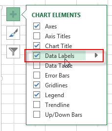
Chart data labels excel

How to Create a Milestone Chart in Excel in 3 Steps ... Steps to Create a Milestone Chart in Excel. I have split the entire process into three steps to make it easy for you to understand. 1. Set Up Data. You can easily set up your data for this chart. Make sure to arrange your data like below data table. Excel: How to Create a Bubble Chart with Labels - Statology Then click OK and in the Format Data Labels panel on the right side of the screen, uncheck the box next to Y Value and choose Center as Label Position. The following labels will automatically be added to the bubble chart: Step 4: Customize the Bubble Chart. Lastly, feel free to click on individual elements of the chart to add a title, add axis ... How to Add Labels to Scatterplot Points in Excel - Statology Step 3: Add Labels to Points. Next, click anywhere on the chart until a green plus (+) sign appears in the top right corner. Then click Data Labels, then click More Options…. In the Format Data Labels window that appears on the right of the screen, uncheck the box next to Y Value and check the box next to Value From Cells.

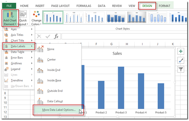
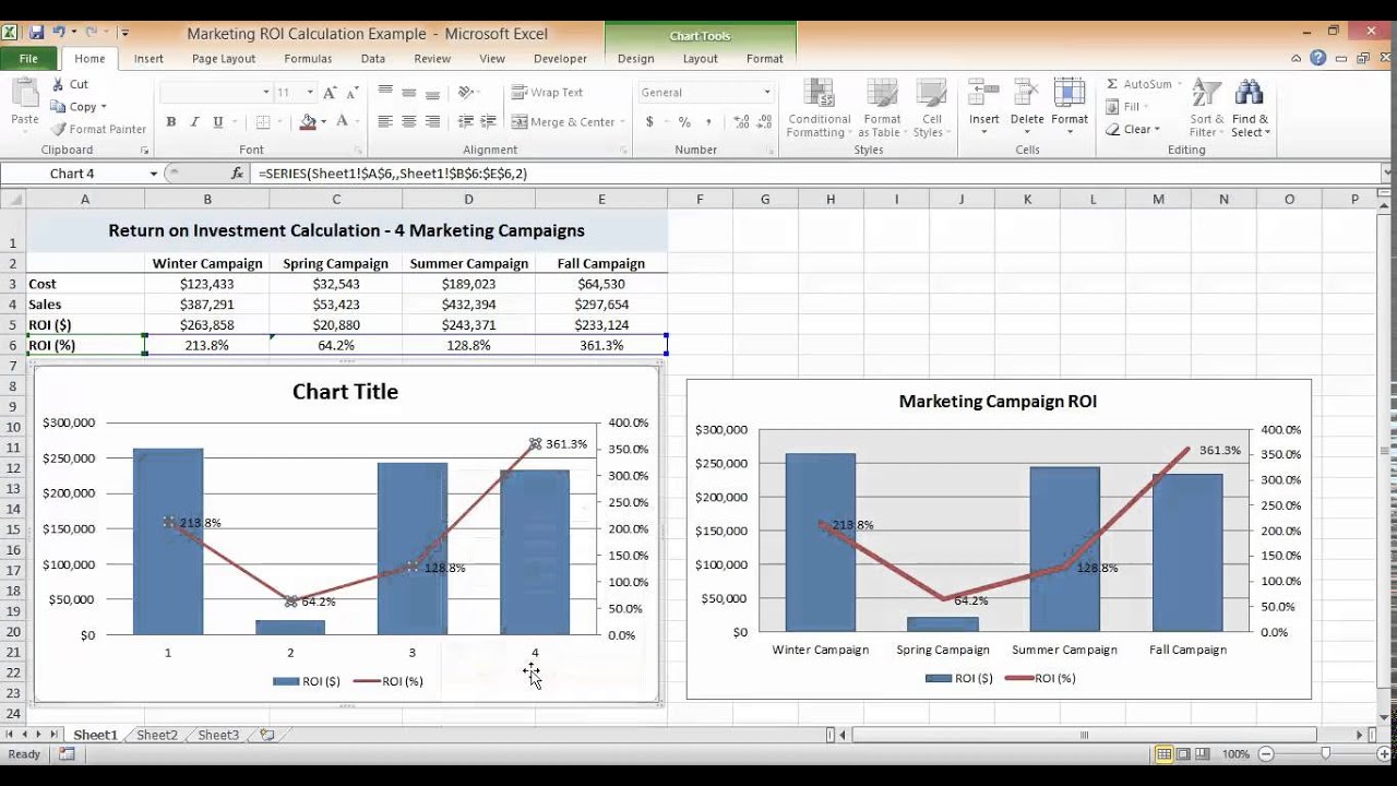
Chart data labels excel. Adding Data Labels to Your Chart (Microsoft Excel) To add data labels in Excel 2013 or Excel 2016, follow these steps: Activate the chart by clicking on it, if necessary. Make sure the Design tab of the ribbon is displayed. (This will appear when the chart is selected.) Click the Add Chart Element drop-down list. Select the Data Labels tool. Chart.ApplyDataLabels method (Excel) | Microsoft Docs For the Chart and Series objects, True if the series has leader lines. Pass a Boolean value to enable or disable the series name for the data label. Pass a Boolean value to enable or disable the category name for the data label. Pass a Boolean value to enable or disable the value for the data label. Add a DATA LABEL to ONE POINT on a chart in Excel | Excel ... Method — add one data label to a chart line Steps shown in the video above:. Click on the chart line to add the data point to. All the data points will be highlighted.; Click again on the single point that you want to add a data label to.; Right-click and select 'Add data label' This is the key step! How to hide zero data labels in chart in Excel? Sometimes, you may add data labels in chart for making the data value more clearly and directly in Excel. But in some cases, there are zero data labels in the chart, and you may want to hide these zero data labels. Here I will tell you a quick way to hide the zero data labels in Excel at once. Hide zero data labels in chart

Custom Data Labels with Colors and Symbols in Excel Charts ... The basic idea behind custom label is to connect each data label to certain cell in the Excel worksheet and so whatever goes in that cell will appear on the chart as data label. So once a data label is connected to a cell, we apply custom number formatting on the cell and the results will show up on chart also. Custom Chart Data Labels In Excel With Formulas Follow the steps below to create the custom data labels. Select the chart label you want to change. In the formula-bar hit = (equals), select the cell reference containing your chart label's data. In this case, the first label is in cell E2. Finally, repeat for all your chart laebls. How to Change Excel Chart Data Labels to Custom Values? First add data labels to the chart (Layout Ribbon > Data Labels) Define the new data label values in a bunch of cells, like this: Now, click on any data label. This will select "all" data labels. Now click once again. At this point excel will select only one data label. Excel tutorial: How to use data labels Generally, the easiest way to show data labels to use the chart elements menu. When you check the box, you'll see data labels appear in the chart. If you have more than one data series, you can select a series first, then turn on data labels for that series only. You can even select a single bar, and show just one data label.

How to create Custom Data Labels in Excel Charts Create the chart as usual. Add default data labels. Click on each unwanted label (using slow double click) and delete it. Select each item where you want the custom label one at a time. Press F2 to move focus to the Formula editing box. Type the equal to sign. Now click on the cell which contains the appropriate label. Adding rich data labels to charts in Excel 2013 ... One familiar and simple way is just single click on any data value (or column, in this example) to select the entire data series that it belongs to. Above, I have clicked all of the blue columns. Once the series is selected, I can right-click any column to pull up the context menu, then click the Add Data Labels entry. Create a multi-level category chart in Excel Select the dots, click the Chart Elements button, and then check the Data Labels box. 23. Right click the data labels and select Format Data Labels from the right-clicking menu. 24. In the Format Data Labels pane, please do as follows. 24.1) Check the Value From Cells box; Excel Chart Data Labels-Modifying Orientation - Microsoft ... Excel Chart Data Labels-Modifying Orientation The chart layout tab has been absorbed into other areas in Excel 2016. I cannot figure out how to change the orientation of the data labels on the axes....(tilt, horizontal, vertical).

Excel Charts - Free Excel Tutorial

Multiple Data Labels on bar chart? - Excel Help Forum Oct 28, 2013 · Apply data labels to series 1 inside end Select A1:D4 and insert a bar chart Select 2 series and delete it Select 2 series, % diff base line, and move to secondary axis Adjust series 2 data references, Value from B2:D2 Category labels from B4:D4 Apply data labels to series 2 outside end select outside end data labels and change from Values to ...

SQL & BI Learning: Pie Chart with data labels outside in ssrs

Actual vs Budget or Target Chart in Excel - Variance on ... Aug 19, 2013 · Set Data Labels to Cell Values Screenshot Excel 2003-2010. The nice part about either of these methods is that the data labels are linked to the values in the cells. If your numbers change or you update the data, the labels will automatically be refreshed and display the correct results. Please let me know if you have any questions.

3d scatter plot for MS Excel

Excel Charts - Aesthetic Data Labels - Tutorialspoint To place the data labels in the chart, follow the steps given below. Step 1 − Click the chart and then click chart elements. Step 2 − Select Data Labels. Click to see the options available for placing the data labels. Step 3 − Click Center to place the data labels at the center of the bubbles. Format a Single Data Label

Excel Custom Chart Labels • My Online Training Hub

Add or remove data labels in a chart - support.microsoft.com Click the data series or chart. To label one data point, after clicking the series, click that data point. In the upper right corner, next to the chart, click Add Chart Element > Data Labels. To change the location, click the arrow, and choose an option. If you want to show your data label inside a text bubble shape, click Data Callout.

Excel charts: Mastering pie charts, bar charts and more | PCWorld

Edit titles or data labels in a chart - support.microsoft.com On a chart, click one time or two times on the data label that you want to link to a corresponding worksheet cell. The first click selects the data labels for the whole data series, and the second click selects the individual data label. Right-click the data label, and then click Format Data Label or Format Data Labels.

E-xcel Tuts: Add Data Labels to Excel Charts

Change the format of data labels in a chart To get there, after adding your data labels, select the data label to format, and then click Chart Elements > Data Labels > More Options. To go to the appropriate area, click one of the four icons ( Fill & Line, Effects, Size & Properties ( Layout & Properties in Outlook or Word), or Label Options) shown here.

Create Charts in Excel - Easy Excel Tutorial

How to add data labels from different column in an Excel ... Right click the data series in the chart, and select Add Data Labels > Add Data Labels from the context menu to add data labels. 2. Click any data label to select all data labels, and then click the specified data label to select it only in the chart. 3.

How-to Use Data Labels from a Range in an Excel Chart - Excel Dashboard Templates

How To Use Dynamic Data Labels To Create Interactive Excel ... If you are an Excel user then this blog is highly useful to you, here know how to create Dynamic Data Labels, which can be highlighted when they are needed the most.. In MS Excel worksheet Chart is a perfect tool to present data in an enhanced and more understandable way but most of the time it is seen that it stuck because of the overloading of the excess of data representation.

Plot Area in Excel and Google Spreadsheets Charts

How to Use Cell Values for Excel Chart Labels Select the chart, choose the "Chart Elements" option, click the "Data Labels" arrow, and then "More Options." Uncheck the "Value" box and check the "Value From Cells" box. Select cells C2:C6 to use for the data label range and then click the "OK" button. The values from these cells are now used for the chart data labels.

Charting in Excel - Adding Data Labels - YouTube

Excel.ChartDataLabel class - Office Add-ins | Microsoft Docs String value that represents the formula of chart data label using A1-style notation. height: Returns the height, in points, of the chart data label. Value is null if the chart data label is not visible. horizontal Alignment: Represents the horizontal alignment for chart data label. See Excel.ChartTextHorizontalAlignment for details.

box-plot-in-excel-3 - DataScience Made Simple

Create Dynamic Chart Data Labels with Slicers - Excel Campus Feb 10, 2016 · Typically a chart will display data labels based on the underlying source data for the chart. In Excel 2013 a new feature called “Value from Cells” was introduced. This feature allows us to specify the a range that we want to use for the labels. Since our data labels will change between a currency ($) and percentage (%) formats, we need a ...

Custom Data Labels with Colors and Symbols in Excel Charts - [How To] - PakAccountants.com

Add / Move Data Labels in Charts - Excel & Google Sheets ... We'll start with the same dataset that we went over in Excel to review how to add and move data labels to charts. Add and Move Data Labels in Google Sheets Double Click Chart Select Customize under Chart Editor Select Series 4. Check Data Labels 5. Select which Position to move the data labels in comparison to the bars.

Pie Chart - PK: An Excel Expert

Adding Data Labels To An Excel Chart | MyExcelOnline Data Labels make an Excel chart easier to understand because they show details about a data series or its individual data points. Depending on what you want to highlight on a chart, you can add labels to one series, all the series (the whole chart), or one data point.

How to create an Excel map chart

How to Add Labels to Scatterplot Points in Excel - Statology Step 3: Add Labels to Points. Next, click anywhere on the chart until a green plus (+) sign appears in the top right corner. Then click Data Labels, then click More Options…. In the Format Data Labels window that appears on the right of the screen, uncheck the box next to Y Value and check the box next to Value From Cells.

Share :