40 data labels excel pie chart

c# - Add data labels to excel pie chart - Stack Overflow I am drawing a pie chart with some data: private void DrawFractionChart(Excel.Worksheet activeSheet, Excel.ChartObjects xlCharts, Excel.Range xRange, Excel.Range yRange) { Excel.ChartObject ... Add data labels to excel pie chart. Ask Question Asked 9 years, 10 months ago. Modified 5 years, 11 months ago. Viewed 9k times Excel 2010 pie chart data labels in case of "Best Fit" Based on my tested in Excel 2010, the data labels in the "Inside" or "Outside" is based on the data source. If the gap between the data is big, the data labels and leader lines is "outside" the chart. And if the gap between the data is small, the data labels and leader lines is "inside" the chart. Regards, George Zhao TechNet Community Support

Edit titles or data labels in a chart - support.microsoft.com On a chart, click one time or two times on the data label that you want to link to a corresponding worksheet cell. The first click selects the data labels for the whole data series, and the second click selects the individual data label. Right-click the data label, and then click Format Data Label or Format Data Labels.

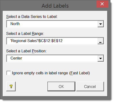
Data labels excel pie chart

Formatting data labels and printing pie charts on Excel for Mac 2019 ... Work around: Select the area of the chart - by selecting the cells behind where the chart is sitting > Print area> Select print area>File > print>then set print perameters (paper size, fit to page etc.) > Print. This worked. 2. When formatting data labels on an extended bar of pie chart: Excel does not allow me to: excel - Prevent overlapping of data labels in pie chart - Stack Overflow However, the client insisted on a pie chart with data labels beside each slice (without legends as well) so I'm not sure what other solutions is there to "prevent overlap". Manually moving the labels wouldn't work as the values in the chart are dynamic. excel Share Improve this question asked Apr 28, 2021 at 2:11 abc 359 3 17 Multiple data labels (in separate locations on chart) You can use the Up/Down arrows to move through chart elements in order to select the second pie. Or use the drop down on the charting toolbar to select the 2nd series Attached Files 819208a.xlsx‎ (77.9 KB, 399 views) Download Register To Reply 08-16-2013, 05:58 AM #6 petesurfer Registered User Join Date 04-16-2013 Location London, England

Data labels excel pie chart. Inserting Data Label in the Color Legend of a pie chart Inserting Data Label in the Color Legend of a pie chart. Hi, I am trying to insert data labels (percentages) as part of the side colored legend, rather than on the pie chart itself, as displayed on the image below. Does Excel offer that option and if so, how can i go about it? Change the format of data labels in a chart To get there, after adding your data labels, select the data label to format, and then click Chart Elements > Data Labels > More Options. To go to the appropriate area, click one of the four icons ( Fill & Line, Effects, Size & Properties ( Layout & Properties in Outlook or Word), or Label Options) shown here. Pie Chart in Excel - Inserting, Formatting, Filters, Data Labels The total of percentages of the data point in the pie chart would be 100% in all cases. Consequently, we can add Data Labels on the pie chart to show the numerical values of the data points. We can use Pie Charts to represent: ratio of population of male and female of a country. proportion of online/offline payment modes of a local car rental ... How to Create Pie Charts in Excel (In Easy Steps) Select the range A1:D1, hold down CTRL and select the range A3:D3. 6. Create the pie chart (repeat steps 2-3). 7. Click the legend at the bottom and press Delete. 8. Select the pie chart. 9. Click the + button on the right side of the chart and click the check box next to Data Labels.

Pie Chart in Excel | How to Create Pie Chart - EDUCBA Step 1: Select the data to go to Insert, click on PIE, and select 3-D pie chart. Step 2: Now, it instantly creates the 3-D pie chart for you. Step 3: Right-click on the pie and select Add Data Labels. This will add all the values we are showing on the slices of the pie. excel - Positioning data labels in pie chart - Stack Overflow Sub tester () Dim se As Series Set se = Totalt.ChartObjects ("Inosa gule").Chart.SeriesCollection ("Grøn pil") se.ApplyDataLabels With se.DataLabels .NumberFormat = "0,0 %" With .Format.Fill .ForeColor.RGB = RGB (255, 255, 255) .Transparency = 0.15 End With .Position = xlLabelPositionCenter End With End Sub Office: Display Data Labels in a Pie Chart - Tech-Recipes 3. In the Chart window, choose the Pie chart option from the list on the left. Next, choose the type of pie chart you want on the right side. 4. Once the chart is inserted into the document, you will notice that there are no data labels. To fix this problem, select the chart, click the plus button near the chart's bounding box on the right ... Make data label colour (pie chart) to match the source cell colour. Hello. I have i pie chart and i want the data labels font colour to match the colour of the source cell. For example i have a category named "shopping" which has a red colour cell. I want the data label on the pie chart to be red.

Add or remove data labels in a chart - support.microsoft.com Click the data series or chart. To label one data point, after clicking the series, click that data point. In the upper right corner, next to the chart, click Add Chart Element > Data Labels. To change the location, click the arrow, and choose an option. If you want to show your data label inside a text bubble shape, click Data Callout. Display data point labels outside a pie chart in a paginated report ... Create a pie chart and display the data labels. Open the Properties pane. On the design surface, click on the pie itself to display the Category properties in the Properties pane. Expand the CustomAttributes node. A list of attributes for the pie chart is displayed. Set the PieLabelStyle property to Outside. Set the PieLineColor property to Black. Is there a way to change the order of Data Labels? Answer. I got your meaning. Please try to double click the the part of the label value, and choose the one you want to show to change the order. * Beware of scammers posting fake support numbers here. * Once complete conversation about this topic, kindly Mark and Vote any replies to benefit others reading this thread. Move data labels - support.microsoft.com Right-click the selection > Chart Elements > Data Labels arrow, and select the placement option you want. Different options are available for different chart types. For example, you can place data labels outside of the data points in a pie chart but not in a column chart.

How to Show Percentages in Stacked Bar and Column Charts in Excel

How to Make a Pie Chart in Excel & Add Rich Data Labels to The Chart! Creating and formatting the Pie Chart 1) Select the data. 2) Go to Insert> Charts> click on the drop-down arrow next to Pie Chart and under 2-D Pie, select the Pie Chart, shown below. 3) Chang the chart title to Breakdown of Errors Made During the Match, by clicking on it and typing the new title.

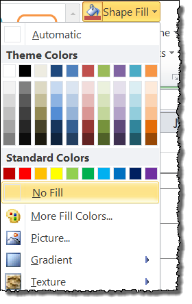
How to Show Percentages in Stacked Bar and Column Charts in Excel

Adding data labels to a Pie Chart in VBA - Automate Excel Learn Excel in Excel - A complete Excel tutorial based entirely inside an Excel spreadsheet. Shortcuts. ... List of all Excel charts. Adding data labels to a Pie Chart in VBA. Excel and VBA Consulting Get a Free Consultation. VBA Code Generator;

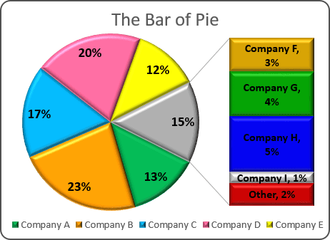
Creating Pie of Pie and Bar of Pie charts - Microsoft Excel 2016

How to display leader lines in pie chart in Excel? - ExtendOffice To display leader lines in pie chart, you just need to check an option then drag the labels out. 1. Click at the chart, and right click to select Format Data Labels from context menu. 2. In the popping Format Data Labels dialog/pane, check Show Leader Lines in the Label Options section. See screenshot: 3.

SQL & BI Learning: Pie Chart with data labels outside in ssrs

Microsoft Excel Tutorials: Add Data Labels to a Pie Chart To add the numbers from our E column (the viewing figures), left click on the pie chart itself to select it: The chart is selected when you can see all those blue circles surrounding it. Now right click the chart. You should get the following menu: From the menu, select Add Data Labels. New data labels will then appear on your chart:

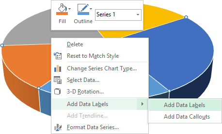
Excel 3-D Pie Charts - Microsoft Excel 2013

Creating Pie Chart and Adding/Formatting Data Labels (Excel) Creating Pie Chart and Adding/Formatting Data Labels (Excel)

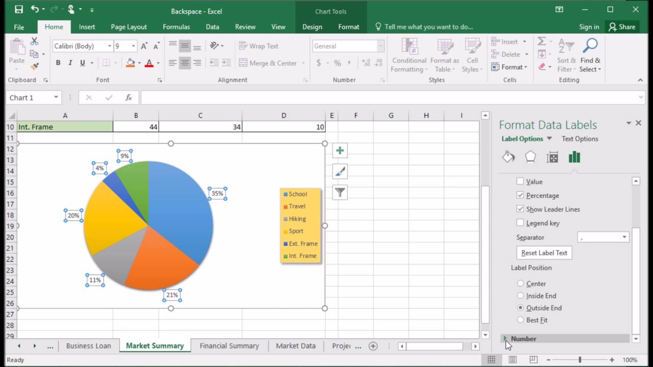
410 How to display percentage labels in pie chart in Excel 2016 - YouTube

How to Create a Pie Chart in Microsoft Excel To create a pie chart, you must first enter your data into the Excel spreadsheet. The data should be entered in rows and columns, with one column for the category name and one for the corresponding percentage or value. Once you have your data set up, select the range of cells that contains it and then click on the Insert tab.

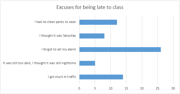
Bar Chart in Excel - Easy Excel Tutorial

Excel Pie Chart Examples - TheRescipes.info Making a Pie Chart in Excel - Brigham Young University-Idaho great content.byui.edu. Step 2: Highlight the data. Highlight the data. If you want to have the labels on the chart, you need to highlight the labels of the data as well.Step 3: In Excel, go to INSERT in the menu.

Python matplotlib Pie Chart

How to fix wrapped data labels in a pie chart - Sage Intelligence Right click on the data label and select Format Data Labels. 2. Select Text Options > Text Box > and un-select Wrap text in shape. 3. The data labels resize to fit all the text on one line. 4. Alternatively, by double-clicking a data label, the handles can be used to resize the label to wrap words as desired. This can be done on all data labels ...

Share :