39 how to add data labels to a pie chart in excel on mac

› 07 › 09Rotate charts in Excel - spin bar, column, pie and line charts Jul 09, 2014 · After being rotated my pie chart in Excel looks neat and well-arranged. Thus, you can see that it's quite easy to rotate an Excel chart to any angle till it looks the way you need. It's helpful for fine-tuning the layout of the labels or making the most important slices stand out. Rotate 3-D charts in Excel: spin pie, column, line and bar charts Pie Chart - legend missing one category (edited to include spreadsheet ... Right click in the chart and press "Select data source". Make sure that the range for "Horizontal (category) axis labels" includes all the labels you want to be included. PS: I'm working on a Mac, so your screens may look a bit different. But you should be able to find the horizontal axis settings as describe above.

How to☝️Create a Pie of Pie Chart in Excel - SpreadsheetDaddy Start off by following the chart creation method as described below. Select your data. Navigate to the Insert menu. In the Chart submenu, click on Insert Pie or Doughnut Chart. Pick the Pie of Pie Chart type. Voila! With those few steps, you have added a Pie of Pie Chart to your worksheet.

How to add data labels to a pie chart in excel on mac

How to Apply a Filter to a Chart in Microsoft Excel - How-To Geek Go to the Home tab, click the Sort & Filter drop-down arrow in the ribbon, and choose "Filter.". Click the arrow at the top of the column for the chart data you want to filter. Use the Filter section of the pop-up box to filter by color, condition, or value. When you finish, click "Apply Filter" or check the box for Auto Apply to see ... › charts › gauge-templateExcel Gauge Chart Template - Free Download - How to Create Step #7: Add the pointer data into the equation by creating the pie chart. Step #8: Realign the two charts. Step #9: Align the pie chart with the doughnut chart. Step #10: Hide all the slices of the pie chart except the pointer and remove the chart border. Step #11: Add the chart title and labels. How to format the data labels in Excel:Mac 2011 when showing a ... Try clicking on Column or Row you want to set. Go to Format Menu Click cells Click on Currency Change number of places to 0 (zero) (if in accounting do the same thing. _________ Disclaimer: The questions, discussions, opinions, replies & answers I create, are solely mine and mine alone, and do not reflect upon my position as a Community Moderator.

How to add data labels to a pie chart in excel on mac. How to Add Data Labels to an Excel 2010 Chart - dummies On the Chart Tools Layout tab, click Data Labels→More Data Label Options. The Format Data Labels dialog box appears. You can use the options on the Label Options, Number, Fill, Border Color, Border Styles, Shadow, Glow and Soft Edges, 3-D Format, and Alignment tabs to customize the appearance and position of the data labels. How to Make a Pie Chart in Excel & Add Rich Data Labels to The Chart! Creating and formatting the Pie Chart. 1) Select the data. 2) Go to Insert> Charts> click on the drop-down arrow next to Pie Chart and under 2-D Pie, select the Pie Chart, shown below. 3) Chang the chart title to Breakdown of Errors Made During the Match, by clicking on it and typing the new title. How to make a pie chart in excel with data - lazylop Locate the Chart panel, and the Pie item:.Click the Insert menu at the top of Excel.Click inside cell E4 and change "Millions" to ITV, if you already have the data from a previous lesson.If you don't have this data, create the following simple spreadsheet. You've created a 2D chart with the BBC data. › 2014/01/20 › excel-chart-titleHow to add titles to Excel charts in a minute. - Ablebits.com Jan 20, 2014 · In Excel 2013 the CHART TOOLS include 2 tabs: DESIGN and FORMAT. Click on the DESIGN tab. Open the drop-down menu named Add Chart Element in the Chart Layouts group. If you work in Excel 2010, go to the Labels group on the Layout tab. Choose 'Chart Title' and the position where you want your title to display.

How to Make a Pie Chart in Excel - tipsmake.com Add your data to the chart. You'll place prospective pie chart sections' labels in the A column and those sections' values in the B column. For the budget example above, you might write "Car Expenses" in A2 and then put "$1000" in B2. The pie chart template will automatically determine percentages for you. Finish adding your data. How to Create a Pie Chart in Excel | Smartsheet If want the category names to appear on or near the chart, right-click on the chart and click Add Data Labels …. By default, the numerical values are added. To add other labels, such as the categorical values or the percentage of the total that each category represents, right-click on the chart, then click Format Data Labels …. How to Make a Pie Chart with Multiple Data in Excel (2 Ways) - ExcelDemy Steps: First, select the entire data set and go to the Insert tab from the ribbon. After that, choose Insert Pie and Doughnut Chart from the Charts group. Afterward, click on the 2nd Pie Chart among the 2-D Pie as marked on the following picture. Now, Excel will instantly create a Pie of Pie Chart in your worksheet. How to make a pie chart in Excel - Ablebits.com For more options, click the Chart Elements button (green cross) at the upper-right corner of your pie chart, click the arrow next to Data Labels, and choose More options… from the context menu. This will open the Format Data Labels pane on the right side of your worksheet. Switch to the Label Options tab, and select the Category Name box.

How To Add A Title To A Chart In Excel For Mac - fasrco This is the result: There is a more complicated way of adding new data into the existing graph through the «DESIGN» «Select Data» menu (open it by right-clicking and selecting «Select Data»). After you click «Add» (legend elements), there will open the row for selecting the range of values. How to reverse axes in an Excel chart? Add a DATA LABEL to ONE POINT on a chart in Excel All the data points will be highlighted. Click again on the single point that you want to add a data label to. Right-click and select ' Add data label '. This is the key step! Right-click again on the data point itself (not the label) and select ' Format data label '. You can now configure the label as required — select the content of ... How to add or move data labels in Excel chart? - ExtendOffice To add or move data labels in a chart, you can do as below steps: In Excel 2013 or 2016. 1. Click the chart to show the Chart Elements button . 2. Then click the Chart Elements, and check Data Labels, then you can click the arrow to choose an option about the data labels in the sub menu. See screenshot: Using Pie Charts and Doughnut Charts in Excel To create one chart of this data, follow these steps: 1. Select the first data range (in this example, B5:C10 ). 2. On the Insert tab, in the Charts group, select the Pie and Doughnut button: In the Pie and Doughnut dropdown list, choose the Doughnut chart. 3. Right-click in the chart area and do one of the following: Under Chart Tools, on the ...

35 Data Label Excel - Labels For Your Ideas

Excel custom pie chart labels - Microsoft Community Specify (space) as Separator in the Data Labels. Set the Number format of the data labels to Custom, and specify (0%) as Type. --- Kind regards, HansV Report abuse 6 people found this reply helpful · Was this reply helpful? Yes No

How To Make A Cashier Count Chart In Excel : How to make an organizational chart - YouTube : Pie ...

Create a Pie Chart in Excel (In Easy Steps) - Excel Easy Select the pie chart. 9. Click the + button on the right side of the chart and click the check box next to Data Labels. 10. Click the paintbrush icon on the right side of the chart and change the color scheme of the pie chart. Result: 11. Right click the pie chart and click Format Data Labels. 12.

29 Add Axis Label Excel Mac - 1000+ Labels Ideas

Pie Chart in Excel | How to Create Pie Chart - EDUCBA Step 1: Do not select the data; rather, place a cursor outside the data and insert one PIE CHART. Go to the Insert tab and click on a PIE. Step 2: once you click on a 2-D Pie chart, it will insert the blank chart as shown in the below image. Step 3: Right-click on the chart and choose Select Data. Step 4: once you click on Select Data, it will ...

New Charts in Excel 2016 • My Online Training Hub

How to Make a PIE Chart in Excel (Easy Step-by-Step Guide) Here are the steps to format the data label from the Design tab: Select the chart. This will make the Design tab available in the ribbon. In the Design tab, click on the Add Chart Element (it's in the Chart Layouts group). Hover the cursor on the Data Labels option. Select any formatting option from the list.

34 How To Label Graphs In Excel - Labels Design Ideas 2020

How To Do A Pie Chart In Excel For Mac - bestbup Select the data you will create a pie chart based on, click Insert > I nsert Pie or Doughnut Chart > Pie. See screenshot: 2. Then a pie chart is created. Right click the pie chart and select Add Data Labels from the context menu. 3. Now the corresponding values are displayed in the pie slices.

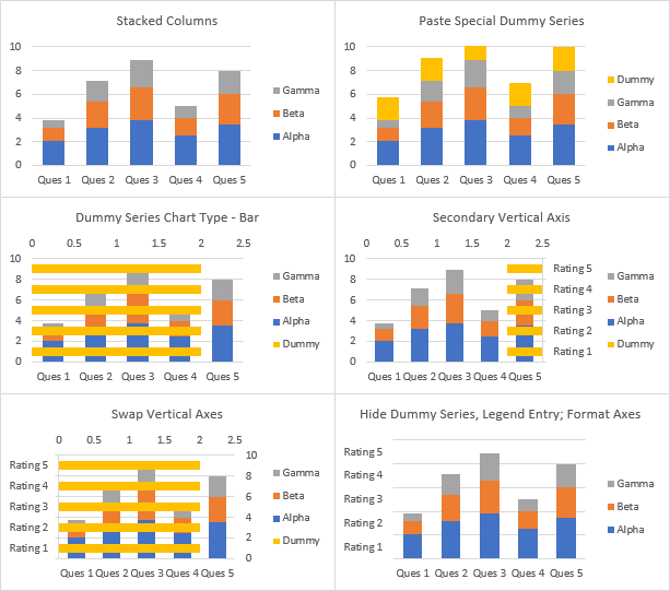
31 How To Label Vertical Axis In Excel

How to Create and Format a Pie Chart in Excel - Lifewire To add data labels to a pie chart: Select the plot area of the pie chart. Right-click the chart. Select Add Data Labels . Select Add Data Labels. In this example, the sales for each cookie is added to the slices of the pie chart. Change Colors

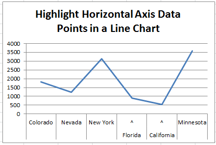
31 How To Label Vertical Axis In Excel

How to display leader lines in pie chart in Excel? - ExtendOffice To display leader lines in pie chart, you just need to check an option then drag the labels out. 1. Click at the chart, and right click to select Format Data Labels from context menu. 2. In the popping Format Data Labels dialog/pane, check Show Leader Lines in the Label Options section. See screenshot: 3.

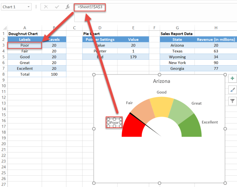
Excel Gauge Chart Template - Free Download - How to Create

› graphs › pie-chartsFree Pie Chart Maker - Make a Pie Chart in Canva Skip the complicated calculations – with Canva’s pie chart generator, you can turn raw data into a finished pie chart in minutes. A simple click will open the data section where you can add values. You can even copy and paste the data from a spreadsheet. Click the text to edit the labels.

Share :